Monitoring Earth through Remote Sensing

Significant shifts in human civilization came from being able to understand patterns in our environment and use them to our advantage. The agricultural and industrial revolutions began with an intution about the seasonal rainfall and the life cycle of plants. Sailors were able to harness the regular flows of the trade winds to make the world traversable in just under 2 years. Today, we have communication systems that can continuously image the Earth for monitoring and understanding. The National Oceanic and Atmospheric (NOAA) collects data for monitoring and assessing the situation of our oceans and climate. For example, the Climate Forecast System drives insight by maintaining high quality measurements of the planet at a half-degree resolution. [1] Now it is becoming cost-efficient to launch new instruments in weather balloons and cube satellites. With the aid of a computer, we can observe environment around us without having to rely on our physical senses.

The sensory adaptions formed out of biological systems. Bats and dolphins use echolocation to map their environment where eyes would typically fail. They can detect slight shifts in the pitch of the sound as it bounces back from moving objects. We have been able to apply our understanding of this Doppler effect to map the earth’s oceans and surfaces through ship, plane, and satellite. The Sentinel-1 constellation [2] collects high-resolution synthetic-aperture radar (SAR) imagery that can track icebergs and map oil spills. This data-driven awareness provides the option to act through increased understanding of interactions and patterns.

A Parallel Programming Model

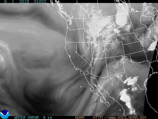Figure: A map of water moisture and cloud cover from the NOAA

Analysis of the data requires a network of computers to run in a reasonable length of time. A recent study of high-performance computing (HPC) software used data from the Climate Forecast System at a 360 x 720 x 41 (latitude x longitude x depth) by 6-hour resolution yielding a 2.2TB matrix of known variables. [3] The amount of data is even higher if we consider imaging data, like the earth view of Google Maps. Planet [4], a San Francisco startup, uses a cube satellite constellation to collect over 5TB of images everyday. Fortunately, the infrastructure to support computational needs are become more mature.

Graphics and Tensor Processing Units (GPUs and TPUs) have become commonplace in computer vision and neural networks. The abundance and regularity of data have fueled the growth of more efficient hardware. The number of floating point operations per second (FLOPS) reflects the efficiency of a processing unit. The global flux of FLOPS has increased through GPUs to support demand for digital processing needs. The GPU started as a dedicated coprocessor designed to paint an image to a screen quickly. Designed to perform basic image manipulation tasks, they formed the basis for general-purpose computing on GPUs.

General-purpose computing on GPUs uses linear algebra to exploit inherent data parallelism. Computer vision libraries like OpenCV use a parallel programming model to write efficient, real time applications. Images are stored in a matrix from where pixels can be manipulated individually or in groups. Linear operators like convolutions can be applied efficiently to filter or transform images. Convoluting an image with an edge-detection kernel produces another image where the values represent the likelihood of being an edge. Machine learning libraries like TensorFlow can also use parallel hardware to speed up computations. TensorFlow now supports TPU coprocessors because of the regularity of convolutions in machine learning applications.[5] The programming interface is more powerful than the hardware it supports, so it’s likely that more efficient hardware will be built.

Figure: An image and the image convolved with an edge-detection kernel. From Kernel (Image Processing), Wikimedia Commons

Distributed data processing libraries like Spark have reduced the complexity of managing powerful computing clusters. By utilizing a network of computers and available global mapping information, we can build systems to detect changes on a large scale. For example, satellite imagery can be used to determine areas of conservation based on historical patterns of deforestation in the Southern Tropic. [6] There are many techniques for processing large datasets, but one particularly efficient one is to treat image data as spectral data. The colors and intensity of an image can be used to extract meaningful patterns. Sometimes infrared and ultrasonic waves are measured in a process called hyperspectral imaging. The spectrum recorded to a map, where every group of observations has a neighbor. This data has a natural grid-like form, where little effort is necessary to parallelize processing.

Finding Patterns in Earth’s Image

With a full image of the surface of the earth, we can start to ask questions about the state of the environment. For example, a health model of the earth may include a distribution of terrain and how they change over time. The global image is broken into common areas and categorized based on its properties. One method is to segment areas of high contrast using the convolution operator and edge-detection kernel. However, the convolution algorithm requires time proportional to the product of the image and kernel dimensions. The convolution theorem helps us bound this operation by replacing an expensive convolution with an efficient change of base and multiplication. This theorem is the foundation for efficient signals processing techniques.

Figure: The convolution of a box signal with itself runs in time proportional to the product of discrete samples from each signal. From Wikimedia Commons.

In space, we can use this to look at the spectrum of different stars. The Fourier transform reveals can reveal the range and intensities of star radiation in a hyperspectral image of the night sky. Discontinuities in this data define the terrain of the sky, where areas are divided by similarity in space and radiation properties. The fast Fourier transform (FFT) calculates an orthonormal base in the frequency domain in order n*log(n) time complexity where n is the product of image dimensions. Because of its efficiency and broad scientific use, the FFT has been described as “the most important numerical algorithm in our lifetime.” [7] This process of transforming between domains is useful for mastering the shortcomings of different techniques.

Graphs are a discrete data structure that can be represented in coordinate and matrix form. In general, most data is discrete because we can’t sample at infinite precision. We can use these individual measurements to describe physical behavior in the form of formulas. Graphs can be used to model physical systems because discrete observations are often related in space or time. Images can form a graphical model where groups of neighboring pixels are connected if they share a common property. This topological approach can be used to build spectral and graphical models for clustering and segmentation.

The spatial image of a graph, known as the Laplacian matrix, is obtained by removing the diagonals of an adjacency matrix. Spectral analysis tools are effective because the eigenvectors of this matrix have a similar interpretation to the Fourier transform. [8] Spectral decomposition is extensively practiced because of algorithms that can process trillions of sparse relations. For example, the PageRank algorithm pioneered by Google uses a method called power iteration to find the eigenvalues of the web hyperlink matrix.[9] Clusters are formed by finding discontinuities in the decomposed form corresponding to graph cuts. This geometrical view of data enables short-cuts for otherwise convoluted solutions.

Figure: The effect of regularization on sparsity in a logistic regression of the MNIST dataset from scikit-learn

Detection is the first step in being able to handle the influx of new sensory data. In addition to being able to determine the lay of the land and contrast different areas, we are often interested in being able to forecast a particular event into the future. The weather forecast is often done by analyzing data over a large area in small cells and modeling the complex dynamical system. The broader problem of forecasting from many, high-resolution streams of data falls under high-dimensional time series analysis. The Climate Forecast System is one example, where each dimension represents a variable or state. However, analyzing thousands of variables at the same time is difficult for most time-series algorithms. [10] One way to tackle this problem is to aggregate streams of data together by clustering similar series. Inducing sparsity in the precision matrix can remove spurious relationships between series, while the eigenvectors of the covariance matrix aid in clustering.[11]

Thoughts

Figure: A simulation of precipitable water from the NOAA

In practice, the complexity of the data with our current computational resources prevents us from producing confident weather forecasts beyond a few weeks. Despite the growing amount of available information, computational power and domain intuition are still limiting resources. However, models driven by massive data have bootstrapped a feedback loop necessary for discovery and refinement. In particular, there are ways to exploit the geometry of spatial data to increase the overall knowledge about the state of the earth. When paired with standard techniques for dimensionality reduction and time series, remote sensing becomes a tool that can help chart a path to coexistence with our environment.

References

[1] Saha, S., Moorthi, S., Pan, H. L., Wu, X., Wang, J., Nadiga, S., … & Liu, H. (2010). The NCEP climate forecast system reanalysis. Bulletin of the American Meteorological Society, 91(8), 1015-1058.

[2] Sentinel-1 - ESA EO Missions - Earth Online - ESA. (n.d.). Retrieved June 1, 2018, from https://earth.esa.int/web/guest/missions/esa-operational-eo-missions/sentinel-1

[3] Gittens, A., Devarakonda, A., Racah, E., Ringenburg, M., Gerhardt, L., Kottalam, J., … & Sharma, P. (2016, December). Matrix factorizations at scale: A comparison of scientific data analytics in Spark and C+ MPI using three case studies. In Big Data (Big Data), 2016 IEEE International Conference on (pp. 204-213). IEEE.

[4] Planet — Platform. (2018, May 07). Retrieved May 31, 2018, from https://www.planet.com/products/platform/

[5] Jouppi, N. P., Young, C., Patil, N., Patterson, D., Agrawal, G., Bajwa, R., … & Boyle, R. (2017, June). In-datacenter performance analysis of a tensor processing unit. In Proceedings of the 44th Annual International Symposium on Computer Architecture (pp. 1-12). ACM.

[6] Allnutt, T. F., Asner, G. P., Golden, C. D., & Powell, G. V. (2013). Mapping recent deforestation and forest disturbance in northeastern Madagascar. Tropical Conservation Science, 6(1), 1-15.

[7] Schneider, D. (2012, February 24). A Faster Fast Fourier Transform. Retrieved June 1, 2018, from https://spectrum.ieee.org/computing/software/a-faster-fast-fourier-transform

[8] Pavez, E., & Ortega, A. (2016, March). Generalized Laplacian precision matrix estimation for graph signal processing. In Acoustics, Speech and Signal Processing (ICASSP), 2016 IEEE International Conference on (pp. 6350-6354). IEEE.

[9] Page, L., Brin, S., Motwani, R., & Winograd, T. (1998). The pagerank citation ranking: Bringing order to the web.

[10] Yu, H. F., Rao, N., & Dhillon, I. S. (2016). Temporal regularized matrix factorization for high-dimensional time series prediction. In Advances in neural information processing systems (pp. 847-855).

[11] Gramfort, A., Blondel, M., & Mueller, A. (n.d.). L1 Penalty and Sparsity in Logistic Regression¶. Retrieved June 1, 2018, from http://scikit-learn.org/stable/auto_examples/linear_model/plot_logistic_l1_l2_sparsity.html